
About 3 decades ago, a shift began in financial planning from modeling investment returns as constant, using straight-line appreciation and time-value-of-money calculations, to variable and uncertain, using historical or Monte Carlo simulations. This was an important step that allowed financial advisors to take sequence-of-returns risk seriously. However, somehow inflation got left out of this evolution in planning analytics.
While investment returns are now treated as varying in almost all widely used financial planning software, inflation is still almost universally modeled using straight-line methods. Investment returns vary across the hundreds or thousands of simulated scenarios that an advisor may use in a financial planning analysis, but the effect of inflation on a plan’s cash flows is exactly the same in every month of every year of every one of those scenarios.
What results is an analytical Frankenstein’s monster: Investments are treated as uncertain and risky, but inflation is modeled as known and risk-free. However, given the elevated inflation rates we have seen recently in the United States, with rates hitting over 9% in 2022, now is a great time to re-examine the need to treat inflation more realistically in financial planning.
Inflation Isn’t Steady And Certain
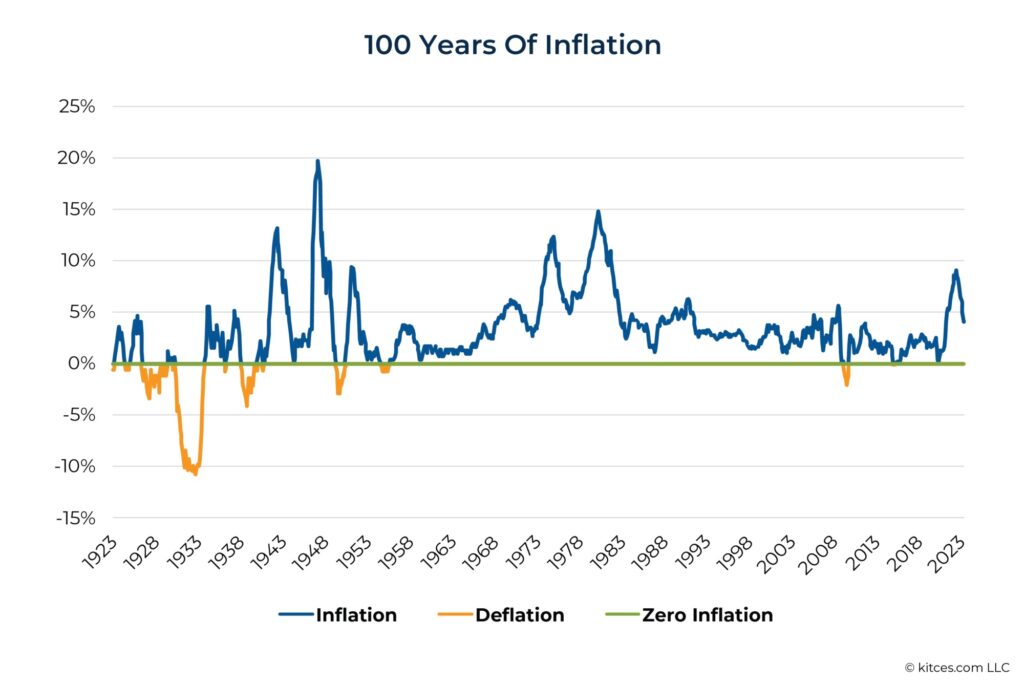
Historically, inflation has certainly not been steady, and it seems unlikely that this will change in the future. Even within the lives of today’s second graders, the US has seen both mild deflation (2015) and inflation of over 9% (2022). Many of today’s financial planners have lived through inflation as high as 14.8% (1980) and deflation of 2% (2009). Most people will recall the feeling, in the decade of 2010–2020, that high inflation seemed a thing of the past, only to see a rapid rise of inflation as high as 9.1% in 2022. Inflation can and does change.
Unfortunately, treating inflation as a constant in financial planning analysis not only misses the mark when compared to history, it can also lead to serious planning missteps with plans that are particularly susceptible to inflation risk. The sequence of inflation rates over time has a direct impact on purchasing power and, depending on how much a plan depends on portfolio withdrawals, can also impact an investor’s portfolio. For example, high inflation levels early in the distribution period of a retirement portfolio can deplete assets more quickly than if inflation rates were lower, and insufficient growth of the portfolio to recover from high inflation periods afterward can compromise the success of the plan. Furthermore, plans that include non-portfolio income that is not adjusted for inflation will suffer more if inflation is higher than expected. As we’ll see below, failing to consider different possible sequences of inflation can lead advisors to miss weaknesses that a plan might have if inflation differs from the assumed rate.
Importantly, while the oversimplification of inflation can impair financial advice, there are other approaches that can potentially help advisors address this problem.
An Example Of “Sequence-Of-Inflation” Risk
When there is risk in a financial plan, financial analysis typically provides a range of options to choose from, each option differing according to how much risk is avoided, transferred, or accepted by following that course of action. This dynamic is familiar from the risk-return trade-off of asset allocation decisions or from the trade-off between withdrawal rates and chance of adjustment in retirement income decisions. But if inflation assumptions are applied at a constant rate, an analysis will provide just one answer to inflation-oriented questions like the ones raised by the following example of a retirement funded with a nominal pension:
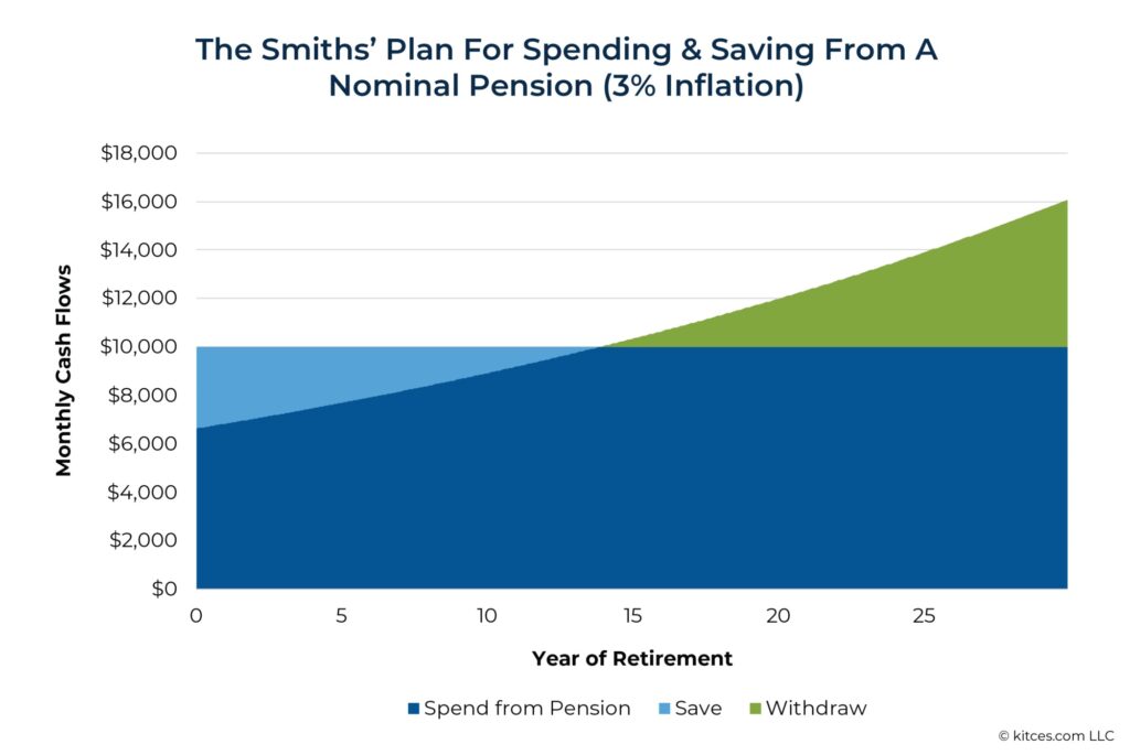
Example 1. The Smith family receives a $10,000 monthly pension payment that is not adjusted for inflation. It is their sole source of income, and they estimate that their retirement will last 30 years. The family’s advisor assumes inflation will be 3% per year.
The Smiths are extremely risk-averse and prefer CDs, savings accounts, and money market accounts. Of course, they are tempted to spend their whole $10,000 pension payment each month, but the advisor knows it would be prudent to have the Smiths put some of their income aside to counteract the future loss of purchasing power due to inflation.
When the family asks their advisor how much they can spend from their income stream, the advisor uses a simple time-value-of-money calculation, assuming the family will first save to and then withdraw from an interest-paying account whose returns will match inflation (i.e., 0% real returns). The advisor estimates that the Smiths can begin retirement by spending just over $6,640/month while saving the other $3,360 and then adjust these amounts for inflation over time.
If the Smiths follow their advisor’s recommendation, will they be able to sustain their real spending through their whole retirement?
While the Smiths in the example above may be dismayed to learn that if they wish to sustain their purchasing power over 30 years in the face of 3% annual inflation, they may have to save more than a third of their pension today to offset future inflation, even this looks like a risky proposition when compared to a full range of historical inflation. During the last 100 years, inflation averaged 2.9%, but actual sequences of inflation would have provided the Smiths with real spending levels as low as $4,350/month (beginning retirement in April 1973).
In the table below, “Historical Success Rate” refers to the proportion of rolling 30-year historical periods that would have supported the sustainable real spending level or higher given actual historical inflation.
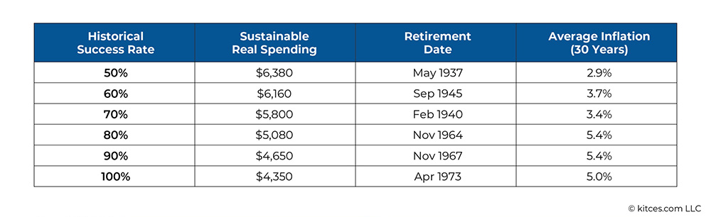
In Example 1, above, the $6,640/month spending level that the Smiths’ advisor would propose when assuming inflation would be a steady 3% per year is higher than even the median spending level that would have been available historically ($6,380/month) over any 30-year period. In other words, if the range of inflation experiences that could occur in the future is anything like the past, it’s probably time to go back to the drawing board for the Smiths.
Inflation isn’t risky simply because it exists – it is risky because it is variable and uncertain. (The same is true of investment returns.) The range of historical answers to this simple planning situation shows how risky and variable inflation has been in the past. The question is, how can we change financial planning analysis to handle inflation more realistically and improve financial advice in the future, especially for clients like the Smiths, who are particularly subject to sequence-of-inflation risk?
Could Higher Fixed Inflation Assumptions Help?
Advisors who only have access to constant inflation modeling (or to systems that allow several inflation constants, each applied to different categories of spending) may wonder if simply assuming a higher fixed inflation rate could help account for inflation risk. Different assumptions for constant inflation will, of course, produce different sustainable spending answers. But it may be surprising how high these inflation assumptions would have to be to produce the range of spending levels for the Smiths from Example 1 that could have survived historical sequences of inflation.
In the case of the Smiths, their sustainable 30-year real spending levels at different historical success rates are indicated in the table below, given their monthly pension income of $10,000 and 0% real return on investments. Next to these, you will see the fixed inflation assumption that an advisor would have to use to produce the same real spending advice.
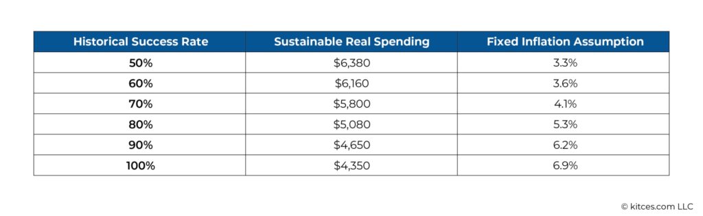
Many of these fixed inflation rate assumptions are higher than may seem reasonable to advisors or clients. To get to 90% historical success, we’d have to assume a constant 6.2% annual inflation rate for 30 years! To handle inflation risk, a fixed inflation rate has to be a lot higher than the expected long-term arithmetic average.
This is analogous to how an advisor who wishes to find a sustainable withdrawal amount from an investment portfolio with varying returns but who uses a constant rate of return and time value of money calculations would have to use a rate of return (much) lower than the expected long-term arithmetic average. For example, assuming a 5% arithmetic average annual real return and 10% standard deviation of returns (not far off from long-term statistics for a 60/40 stock/bond portfolio) in a basic Monte Carlo simulation, a $1,000,000 portfolio could produce roughly $46,700/year for 30 years with an 80% probability of success. To produce this same withdrawal amount using straight-line appreciation, we would have to use a constant 2.3% real rate of return – well below the assumed 5% arithmetic average.
But, of course, this is not what most advisors do when modeling investment returns. Not only would this approach be difficult to explain to clients, it would also fail to provide the client with options. When investment returns are variable and uncertain, choices about portfolio withdrawals reflect retirees’ preferred balance between spending and how much sequence of returns risk they are willing to accept.

Using a constant rate of return and calculating a single spending amount doesn’t present a range of options from which to choose. Only a model with varying returns does that. In the same way, simply assuming a high constant inflation rate doesn’t present choices – it just models a single scenario and produces a single answer.
When faced with variable and uncertain investment returns and evidence that investment risk matters for clients’ financial plans, advisors began including variance of investment returns in their analyses. In the same way, sequence-of-inflation risk can be included in a plan, either by using historical inflation sequences or by adding variance to inflation assumptions in the capital market assumptions deployed to produce Monte Carlo simulations. (Both of these approaches are offered in Income Lab’s retirement income software.)
Treating inflation as variable gives advisors a way to explore a range of inflation experiences for clients like the Smiths from Example 1, and for other client situations where inflation risk is important. Exploring high-inflation, low-inflation, and mixed-inflation scenarios allows advisors to give customized advice that balances clients’ spending and their willingness to take on sequence-of-inflation risk.

Treating Inflation As Variable In Monte Carlo Simulations
History provides a wide range of inflation sequences and potential spending levels for the Smiths, introduced earlier in Example 1. But for those who wish to define their own inflation assumptions, Monte Carlo methods can also be used to model variable inflation (though few software systems offer this option today). If a 3.5% standard deviation is added to the 3% average annual inflation assumption above, a Monte Carlo analysis produces the following range of spending levels (at and above 50% probability of success) for the Smiths.
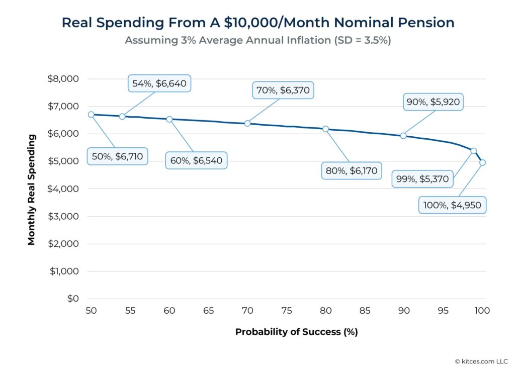
The Smiths’ advisor could, of course, choose to use lower or higher inflation assumptions and get a different range of answers. (The assumption above of a 3.5% standard deviation of inflation was chosen to produce results that resemble those we saw for historical sequences of inflation.) But, spending $6,640/month (the spending level produced in Example 1 above) has a forecasted 54% probability of success in this analysis. In other planning situations, an advisor would be unlikely to propose a plan with a 50% probability of success (though perhaps that’s not as scary as it sounds). Most advisors prefer to target higher probability-of-success levels. In this example, allowing inflation to vary would allow an advisor to do exactly that.
We’ll now turn to an example that shows more clearly how variable inflation can reduce success rates and increase risk forecasts in more complex plans.
Inflation Risk Meets Investment Risk
So far, we’ve focused on an example with a 0% real return assumption that lets us isolate inflation risk. However, many or most retirement plans also depend on withdrawals from investment portfolios. It’s fair to assume that the sequence of returns, rather than the sequence of inflation, could be the overriding concern for these plans. But the question is whether we are in danger of overestimating spending and underestimating risk when using fixed inflation for these plans or whether, instead, the variability built into portfolio returns also handles inflation risk adequately (even if inflation is treated as fixed)? The answer is, “It depends.”
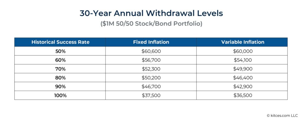
Historical simulations that include variable inflation produce lower sustainable withdrawal levels than those that use fixed inflation at the historical average. The following table shows 30-year annual withdrawals at different historical success rates from a $1 million 50/50 stock/bond portfolio.
It is easier to understand these differences and to compare across examples by asking how risky the spending levels produced by a fixed inflation assumption are when analyzed using variable inflation instead. The graph below shows a trio of paired bars for each level of stock allocation. Each pair represents the probability of success using a fixed inflation assumption (on the left, in blue) and variable inflation (on the right, in green). When the green bar is lower, this shows treating inflation as variable uncovers risk for the plan and decreases that plan’s probability of success.
For example, we see above that withdrawing $46,700/year has a 90% success rate using a fixed inflation rate with a 50/50 stock/bond portfolio. Below, we see in the rightmost pair of bars for 50% stock that when inflation is variable, this same withdrawal level has 79% success.
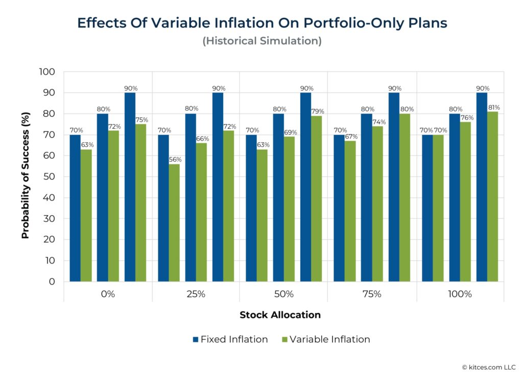
The analytical bang for the buck of adding variance to inflation is clearly not the same for all plans. The impact of including variable inflation depends on the make-up of the portfolio and the level of risk (or probability of success) that an advisor is targeting. For example, we see above that the withdrawals from a 25% stock portfolio that have a 90% success rate using fixed inflation have only 72% success with variable inflation – certainly a meaningful difference. On the other hand, we see no difference at all between fixed and variable inflation for withdrawals from a 100% stock portfolio at a 70% success rate.
Comparing risk levels in this way shows that there are 2 basic patterns at play here:
1. The effect of including variable inflation gets smaller as stock allocations (and thus returns) increase.
2. The effect of including variable inflation is larger at lower risk levels (i.e., higher success rates).
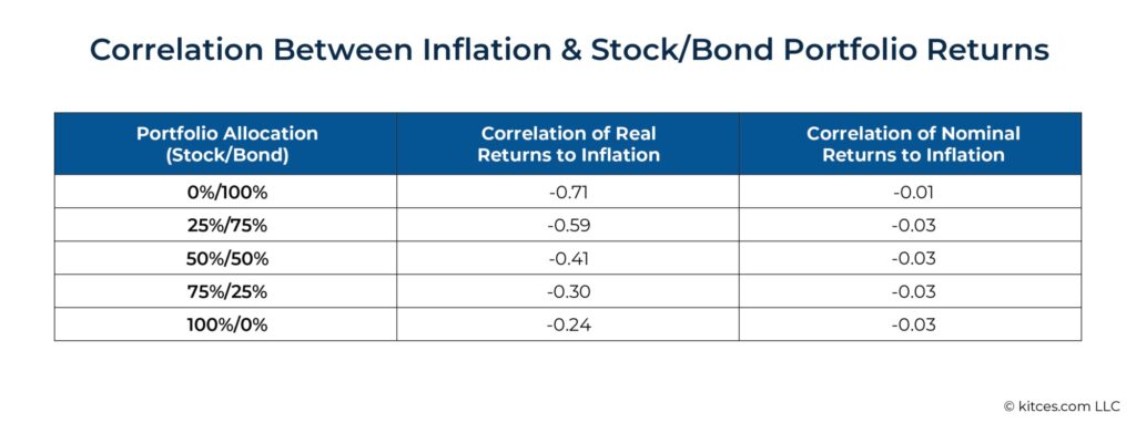
These patterns make sense. First, the real return of bond-heavy (lower return) portfolios is more likely to be affected by inflation. Historically, inflation has a more significant negative correlation to the real returns of bond-heavy portfolios than to stock portfolios. That means that when they encounter worse sequences of inflation, sustainable withdrawals from bond-heavy portfolios suffer more than from stock-heavy portfolios. In other words, returns of stock-heavy portfolios are more likely to absorb the blows of higher inflation.
Second, using variable inflation has a larger effect when targeting lower-risk spending levels (i.e., those associated with higher probabilities of success) because these lower-risk spending levels reflect simulated scenarios that are more likely to involve poor sequences of inflation. On the other hand, when risk is at the median (around 50% probability of success), we’re likely to be observing inflation closer to the average, so variance in inflation won’t have as great an effect.
Nerd Note:
Monte Carlo simulations show a similar pattern to what is shown in the paired bar graph shown earlier (Effects of Variable Inflation On Portfolio-Only Plans) except that, when using standard Monte Carlo methods, the effect of treating inflation as variable quickly disappears as returns rise to 6% (with 3% inflation). In other words, Monte Carlo methods might lead us to conclude that variable inflation doesn’t matter for moderate-to-high return portfolios. However, given what we know from the historical data just discussed, it’s probably best to interpret this more muted impact of variable inflation as an artifact of the standard Monte Carlo methods used in financial planning rather than as permission to ignore variable inflation. Monte Carlo methods that accommodate more complex interactions between and among returns and inflation would be needed to capture the effects seen historically. However, though this would be analytically satisfying, sourcing and managing many additional (complex and arcane) capital market assumptions would likely be impractical. For those who use Monte Carlo methods with variable inflation, it may be prudent to be a bit more conservative in establishing capital market assumptions or in plan selection to counteract the tendency of Monte Carlo methods to understate the effects of variable inflation.
Risk management requires considering how actual outcomes could differ from the expected outcome – especially if those differences could lead to loss. Because inflation is, in fact, variable and uncertain, we know that actual inflation outcomes will differ from simplistic fixed inflation assumptions. Depending on the resources a client brings to retirement, this departure from reality can really hurt.
The following graphic shows how the importance of treating inflation as variable can change depending on a plan’s characteristics, where certain factors (such as lower return expectations and higher probability of success targets) tend to be more sensitive to variable inflation conditions.
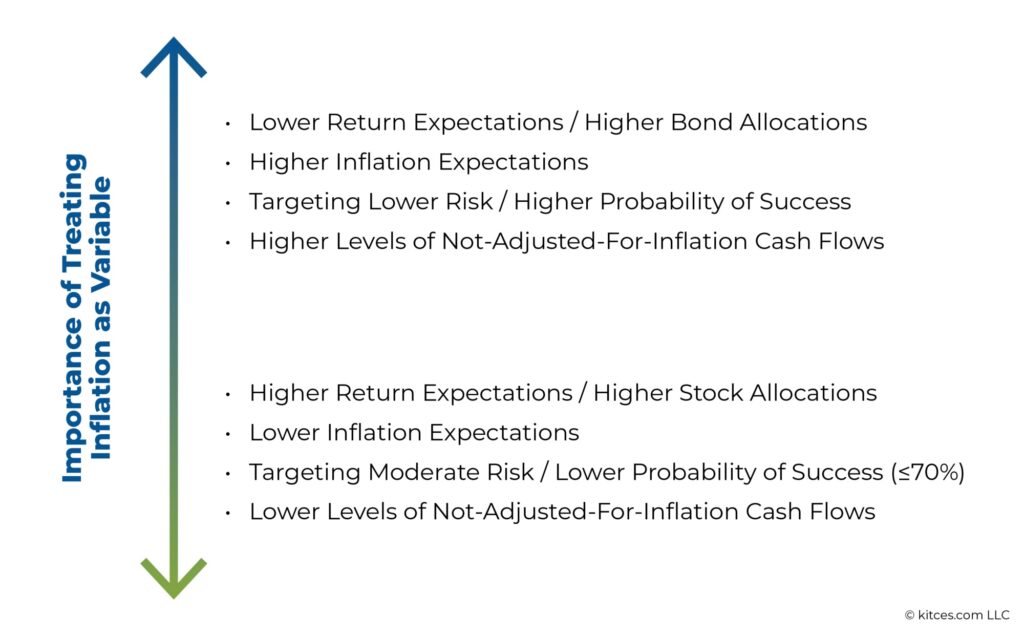
This figure shows that variable inflation analysis has very high value for a plan that, for example, targets an 80% probability of success, has relatively low return assumptions, and has meaningful not-adjusted-for-inflation income (such as from a pension). Treating inflation as fixed is likely to overestimate spending capacity and underestimate risk for this plan. On the other hand, a plan with no not-adjusted-for-inflation income, high return assumptions, and lower probability of success (e.g., 60%) has less to gain from treating inflation as variable and is less likely to overestimate spending and underestimate risk.
Given that options for modeling varying and uncertain inflation exist and that many plans are affected – at least somewhat – by inflation risk that isn’t fully captured when modeling inflation as fixed, it is hard to defend the broad use of fixed inflation assumptions in financial planning.
However, those who do not have access to technology that can treat inflation as variable may wish to target comparatively lower spending levels (and therefore higher probabilities of success), especially when plans have characteristics that are most impacted by variable inflation (e.g., those listed at the top of the figure above).
Ultimately, the key point is that inflation is not fixed and known – it is variable and uncertain. The quality of financial plans and financial advice can suffer when inflation is oversimplified. By treating inflation more realistically, advisors can better understand how inflation affects each financial plan and ensure they are offering the best recommendations for their clients!
The article was originally posted on Kitces.com here.

Continue Reading
Ready to see this in action?
Watch how Income Lab helps advisors answer clients' toughest retirement income questions with guardrails-based planning.
Book a Walkthrough Start Free Trial